Diversifying with Options

“We observe a world of great opportunities disguised as insoluble problems.”

Franklin Roosevelt 1938

Diversifying with Optionality

Volatility and the Short Convexity Trade

Volatility is an often misunderstood and confusing topic.  It is, perhaps, even more misunderstood as it is applied to financial markets.  Traditionally, investors tend to ignore volatility, only acknowledging it when it arises out of nowhere and crashes down like a rogue wave.  But they’re not alone.  Maybe it’s because volatility is nearly impossible to predict and relatively rare, that many market participants try to reason it away or completely discount its long-term impact.  The problem is you can’t ignore it because nearly all investing and financial planning revolves around volatility and its calculated version, standard deviation.  Standard deviation pervades nearly all the investment world.  It is the primary factor in calculating investment risk and determining the success of most financial plans.  It is inescapable.  There’s just one issue, standard deviation is highly flawed. 

Standard deviation is the calculation of how far distributions vary from the mean.  Standard deviation is incorporated in the bell curve’s normal distribution of returns, and the entire financial industry utilizes the bell curve, to some degree, to determine probabilities.  The problem is that the market’s returns are anything but normally distributed.  Well, ok, that is not exactly true.  I’ll give it some credit, it’s like the line from the movie Anchorman, “50% of the time it works all the time.”  Meaning, a good percentage of the time returns are fairly normally distributed.  But then there are those pesky periods, when they’re not.  Those periods are fairly rare, perhaps explaining why they get ignored.  However, the impact from those “rare” times cannot be ignored.  To quote Bruce Springsteen, “from small things, mama, big things one day come.”  While rare, these non-normal returns can be transformative.

One recent example would be the Financial Crisis of 2008-09.  If we analyze the daily returns going back to 1950, according to the bell curve, the S&P 500 should only witness daily moves greater than 5.8% or lower than -5.76% approximately once every 209,000 years.  Yes, you got that right, in the time since modern humans first came into existence, we should have witnessed just one occurrence of the stock market moving greater than 5.75% in either direction.  However, between September 29, 2008 and March 23, 2009 it happened 15 times, or roughly 12.5% of the time!  The chances of that occurring, 15 rogue moves in 120 trading days, is beyond my ability to calculate, but let’s just settle for never.  As tempting as it may be to reason that away as a once in a lifetime, or once in a two hundred millennium occurrence, this frenetic price movement wasn’t exclusive to the Great Financial Crisis.  Since 1987, we’ve seen 9 other such instances.  All told we have had one of these outsized moves about once every 1.5 years. 

So, if the markets returns are not normally distributed, why is it still used to project risk and return?  Well, the fact is that most of the time it fits.  Normal distribution of daily returns on the S&P 500 projects that 95% of the time returns will fall between -1.9% and +1.96%, and as it turns out, actual historical returns showed that 95% of the time returns fell within that range.  Now, this is a little bit of manifest destiny, since the calculation to arrive at these numbers actually implies that it will fit.  Standard deviation is calculated by analyzing actual returns and “getting the math to fit” historical returns.  More precisely, it is not a projection, it is a calculation done in the rear-view mirror.  But still, the 95% confidence level is fairly accurate when projected over any period of time. Where the calculation does start to show cracks is at the extremes.    

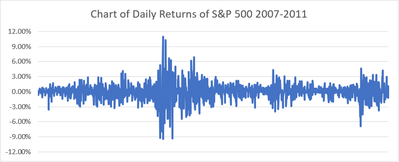
Above are the daily returns of the S&P 500 between Jan. 2007- Dec 2011. Under normal “Bell Curve” distribution, roughly 95% of the daily returns would be between +-2%, and almost never should returns be greater than +-6%.

So, what is the overall impact of these rare, “rogue” events?  The cumulative returns of the “rogue” down days since 1987 is -121%.  Even when allowing for the “rogue” up days, the total returns since 1987 were nearly half what they would’ve been, had these days that never should’ve been, not have been.  Put in more concrete terms, if you’d invested $100 in January 197 and skipped those days which “should not” have happened you would have over $2145 today, compared to the $1115 you would have by buying and holding.  Finally, consider for a minute, the impact that this difference has upon your future retirement plans.  If the financial plan you ran with your financial advisor projected your success based upon a normal distribution of returns, chances are that those returns are too generous, and your chances of outliving your money are higher than you may think.  Similarly, the same issues exist with many pension funds relying generously on higher returns, lower volatility, and ignoring extreme non-normal returns.  Ignoring extreme events because they are rare is like ignoring human existence because the chances of it happening were extremely rare.  Paradoxically, improbable events are the most transformative.

Predicting the Unpredictable, or Seeking Shelter from Convexity

One reason why so many market participants discount extreme events in the stock market is because of the seemingly futile exercise of trying to predict their occurrences.  Prediction is hard.  While predicting the common, everyday events is slightly conceivable, predicting the rare event is nearly impossible.  But does our inability to predict these events mean we should just ignore them?  How does diversification help reduce our overall exposure to rare events?  Diversifying across asset classes may help reduce the impact of one asset class experiencing a tail event, but it hasn’t always shown the best results protecting portfolios in times of financial crisis, especially over shorter time horizons.  When we look back at those dramatic trading days, starting with the October ’87 market crash, we can clearly see the limits of asset diversification. 

*Diversification benefits shows the excess return between a portfolio of 60% stock/ 40% bonds and a portfolio of 60% stock/ 40% cash.

We see that, on these days, bonds did not react with nearly the same magnitude as stocks, and in some cases bond prices declined, in tandem with stocks.  Diversification benefits are really more effective within the 95% confidence range of the bell curve.  Smaller, more incremental losses in share prices can more reliably be buffered by bond price action, but standard bond allocations provide very little support during the deluge of severe market corrections.

Market timing is also a well-documented poor option for loss protection.  Hopping in and out of the market tends to lead people to exiting and entering the market at the wrong times.  Relying on market valuations to guide our decisions to enter and exit can also prove difficult.  Robert Shiller, Nobel Laureate and creator the Cyclically Adjusted PE Ratio, has readily admitted his creation is a poor tool for market timing.  CAPE levels higher than 25 are typically associated with high levels of market exuberance, only having been eclipsed 4 times (1929, 1995, 2004, and currently since 2014).  However, in recent years, exiting at elevated P/E level would’ve been seen as premature.  The CAPE PE breached 25 in December 1995 with the S&P 500 trading around 615, by the time the market peaked in 2000 it was trading above 1500, 143% higher than when it first became “overvalued.” In 2004, the PE again eclipsed 25 with the S&P trading around 1100 before peaking again at 1500, or 36% higher.  Finally, in 2014 it overtook 25 again, this time with the S&P 500 trading at around 1960, currently the S&P 500 sits at roughly 2750, 40% higher.  This isn’t meant to diminish Mr. Shiller’s work, it is only meant to show that basing investment decisions on valuations can be extremely costly.           

So, the question remains, if predicting these events is relatively impossible, and if diversification benefits are muted in times of crisis, must we be resigned to trudging on in the face of obvious peril, with our only comfort being the fact that most likely it isn’t lethal, or is there another way to improve our situation.  Can we find a systematic method, independent upon guessing or predicting, that can protect us during these transformative market events?  One possible approach would be to adjust how we look at asset allocation and diversification.  Instead of segregating assets according to asset class, another approach would be to analyze them according to convexity, or gamma.  Gamma and convexity are interchangeable words in options trading to define the investment payoff of an option or option strategy.  For our purposes it would be best to confine the discussion to its relationship to our pesky problem of non-normal return distributions.   

Imagine the curvature of spoon.  The backside of the spoon is peaked in the middle and slopes downward towards the edges.  This is what we commonly know as a convex shape, but in the investment world this is referred to as negative convexity.  The other side of the spoon, where your food sits, is concave, or positive convexity.  Positive convexity, or long gamma, is more unique in the investing by the nature of its payoff.  Positive convexity profits from things being different than they are currently.  Positive convexity prefers disorder rather than order.  When you are long option gamma, what concerns you is not so much the direction a stock moves, but how much it moves.  Radical price movement is the friend of long gamma.  On the flip side, when you are short gamma, or exhibiting negative convexity, you prefer orderly price movement, and prefer things similar to the way they are currently. 

Most investments exhibit short convexity, because most investments prefer life inside the bell curve.  Normalcy is preferred whether you are long the stock market or invested in a diversified asset allocation strategy; normalcy meaning you want things to go according to plan.  Traditional diversification demands that correlation levels abide by historical norms and do not vary far from the historical range.  Our earlier discussion of the historical dramatic stock market events clearly tells you that you want things normal rather than abnormal.  The more returns stay within the 95% confidence level of the bell curve, the better the returns will be for short convexity investments.  

Life outside the normal distribution of the bell curve, on the other hand, is desired only by those investments with positive convexity.  Traditional asset allocation strategies rely on correlation to balance risk.  Combining stocks and bonds to create a portfolio balance like 60% stock/40% bonds for a conservative growth allocation can seem prudent given that government treasury bonds and stocks tend to be negatively correlated, or at least not correlated at all.  Combining these assets together can create a portfolio that adequately weathers the storm during normal periods--again inside the bell curve.  However, each of these assets by itself is a negative convexity investment, and combining them, unlike the laws of physics, does not make a positive convexity allocation strategy.    

If diversifying between asset classes fails to adequately protect us during those periods of dramatic price drops, can we improve our method of diversification?  Perhaps building a more durable portfolio can be attained by adding a little positive convexity to the mix.              

Long Convexity:  The Added Power of Exponential Returns

The true power of a long gamma or a positive convexity trade is its ability to provide exponential returns with finite loss exposure.  Compared to a long stock or long bond positions, which have linear returns, long gamma trade’s returns are significantly higher than its maximum loss.  Below are some examples of positive convexity trades:

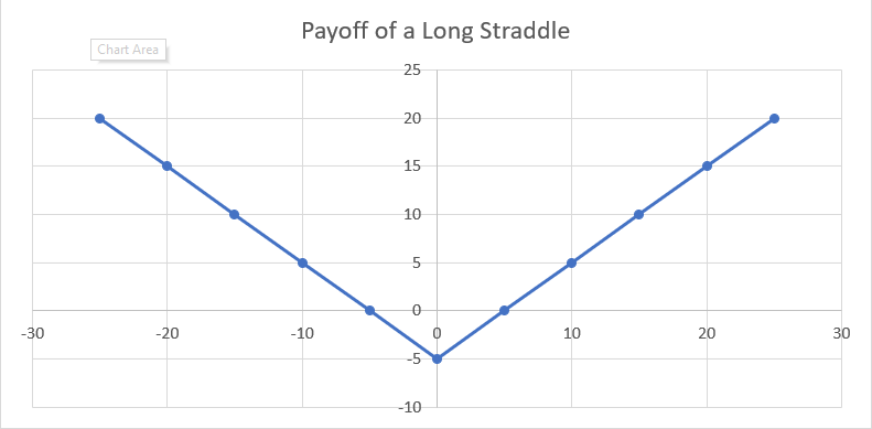
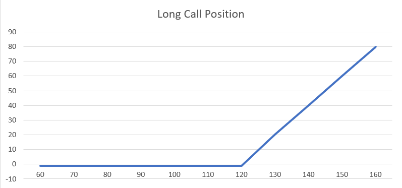
The common thread being controlled risk with the potential for outsized returns.  This is the nature of positive convexity.

 Another example of positive convexity is the relationship between the Cboe Volatility Index and the S&P 500 Index.  The VIX Index is a measurement of the implied volatility on the 30 day S&P 500 options. The VIX Index exhibits convexity because its rate of change is exponentially inversely correlated to the rate of change of the S&P 500.  Typically, it is assumed that the VIX Index rises 5% for every 1% that the S&P 500 declines.  However, the 5:1 relationship is an average; therefore, it too is prone to the same errors of normal distribution.  During more extreme periods we should expect this relationship to behave erratically.  For example, on February 5, 2018 the S&P 500 dropped a little over 4%, simultaneously the VIX Index rose over 115%.  At 29:1 the rate of change far eclipsed its traditional 5:1 ratio.  One would have to wonder what the VIX reaction would be if we had a repeat of the October 1987 Crash.  Even at a more modest 15:1 ratio, a 20% decline in the stock market would imply a 300% increase in the VIX.

These examples are meant to serve as illustrations of positive convexity.  The value of adding such an allocation provides, not just exposure to investments that are negatively correlated to traditional investments, but also the ability to receive exponential returns in exchange. Positive convexity allows us to make smaller, incremental allocations which can ultimately provide larger, substantial support during times of crisis in the market.  If bonds have provided only fractional support during previous days of large stock market losses, it seems almost necessary to add alternative measures of defending oneself. 

There Ain’t No Such Thing as a Free Lunch

Positive convexity trades come at a cost.  Like most insurance policies they have premiums that have to be paid.  Also, like insurance premiums the cost of insuring goes up as the perceived chances for disaster go up. Additionally, because dramatic drops in the stock market can arise seemingly out of nowhere, it becomes nearly impossible to time your protection purchase.  Investment which capitalize on disorder or events “outside the bell curve,” require nearly systematic allocation.  Imagine canceling your health insurance 5 days before you had a major health problem.  Not only will the hospital bills kill you, but you will have wasted all the money you previously spent on premiums. 

The more vanilla hedging strategies can either be cost prohibitive or provide insufficient protection.  Currently[1], the cost of an at-the-money put expiring in 52 days on the S&P 500 cash index is nearly 2% of the index value.  Consistently paying 2% every two months, to hedge an investment which has an average return of 9% is clearly not something anyone should do.  Even if you purchased a put providing one year of protection, the cost would be over 5.5%. 

What about a vanilla strategy on the VIX Index?  Currently a three week at-the-money call option is over 11% of the VIX Index value.  So, simply buying a VIX call option would also be cost prohibitive.  Building a positive convexity strategy is not something that can easily put together.  It requires expertise and understanding, not just about options, but about the nature of convexity investments.  At Calibrate Wealth, we have the necessary expertise to build a sophisticated convexity investment that can help you weather the market storms that seek to derail your investment goals.  We would welcome the opportunity to discuss ways in which we can protect your investment portfolio and help you achieve financial goals.  Come discover the Calibrate difference.